You may be wondering, “What is the VLOOKUP function, and why should I bother learning it?” Well, as it turns out, this is one of the most used Excel functions, and understanding how to use VLOOKUP will yield great benefits.
I’ll try to keep this article as simple as possible. Think of it as VLOOKUP for dummies 🙂
Contents hideVLOOKUP is used to search and retrieve data from a specific column in a table. For example, you can look up the price of a product in a database or find an employee’s name based on their employee ID.
Approximate and exact matching is supported, and wildcards (* ?) can be used for partial matches.
The first questions I hear from people are “how does VLOOKUP work?” and “how to do VLOOKUP?” The function retrieves a lookup value from a table array by matching the criteria in the first column. The lookup columns (the columns from where we want to retrieve data) must be placed to the right.
It’s important to understand the VLOOKUP function syntax. There are four arguments:
=VLOOKUP(lookup_value, table_array, col_index_num, match_type)
lookup_value: the value you are trying to find in the first column of the table
table_array: the table containing the data (the Excel lookup table)
col_index_num: the column number in the table that contains the value you want to return
match_type: true = approximate match; false = exact match
I strongly recommend downloading the free Excel VLOOKUP example file, as this VLOOKUP tutorial will be based on the data provided inside.
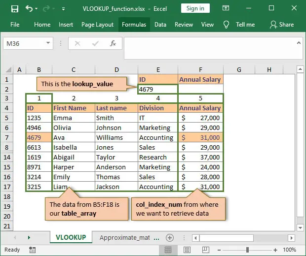
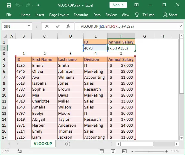
The first step in understanding how to write a VLOOKUP formula is identifying which data you need to retrieve. In this case, it is the Annual Salary of the employee with the ID number ‘4679’. This is the lookup value argument. As I mentioned, this value needs to exist in the first column of your table. VLOOKUP performs the search in the first column and retrieves the info from whichever column you specify to the right.
The second step is to select the data where this info is available. In the image above example, this is table B5:F17 and this range is the table array argument.
The third step is to check the column number from where we want to retrieve the info. Remember that this refers to the number of columns from the table array range, not the Excel column number. This is important! Since we need the Annual Salary (stored in column F), we will use 5 as the col_index_num argument.
The final step is to choose Exact match or Approximate match. Because we are looking for a specific employee ID, we need to use Exact match. I can safely say that around 95% of your VLOOKUP formulas will use Exact match. Since the match type parameter is optional, please remember that Excel uses Approximate match by default. If you want to be on the safe side, I strongly recommend that you always input a value for your match_type argument.
Here’s a quick video from Microsoft that demonstrates how to write a VLOOKUP formula.
I’ve also included another video showing two practical VLOOKUP examples. If you have the time, I encourage you to watch it because it shows how to use VLOOKUP with larger data sets.
If you want to learn how to ignore and hide #N/A error in Excel, keep reading. The following chapter teaches you two methods to hide the #N/A VLOOKUP error message.
Sometimes, when you use the VLOOKUP function in Excel, your formula might return the #REF! error message. There are two possible reasons why your VLOOKUP formula is not working: you have invalid range references, or a cell or range referenced in your formula has been deleted.
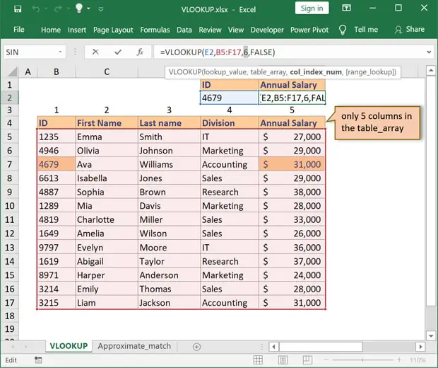
The most common fix is to check your col_index_num parameter. Most likely, the value is higher than the total number of columns in your table.
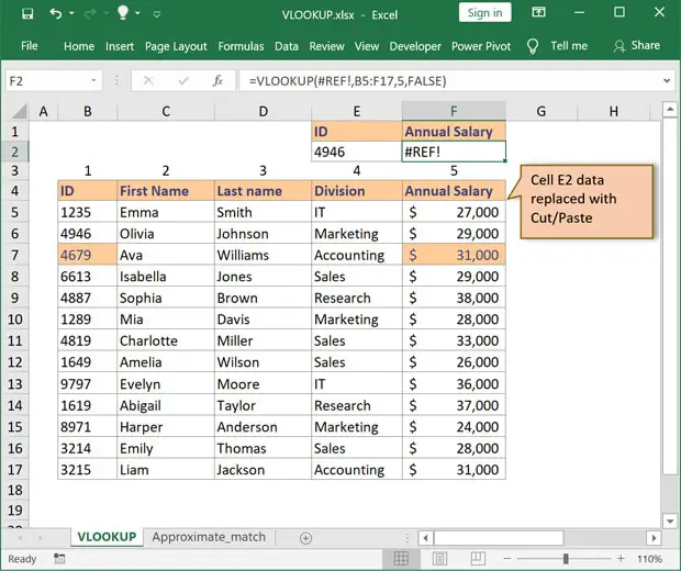
In the formula below, the col_index_num is 6, but there are only 5 columns in the table array. This will get you a #REF! error message.
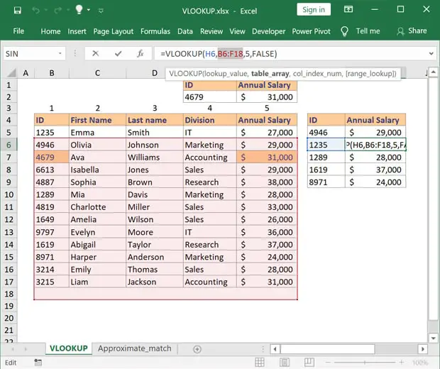
If your formula contains the string #REF! in the formula bar, then it means you have deleted either the lookup value or the table array. Cutting and pasting values in cells linked to your VLOOKUP formulas will trigger the same error message.
The image below shows a VLOOKUP #REF! error generated from cutting and pasting data to cell E2, which is the lookup value.
If this doesn’t fix your VLOOKUP #REF! error, please refer to my #REF error in Excel article.
Whenever I teach someone to use VLOOKUP, I emphasize that a VLOOKUP formula can trigger many errors, but you only want to trap and set a customized error message when VLOOKUP returns the #N/A error. Why is that? Well, that’s because an #N/A error means that the value you are looking for was not found, but a #VALUE error means something completely different.
If you hide all errors behind a custom message, you are doing yourself a huge disservice for two reasons.
Firstly, a function like IFERROR only hides the error but doesn’t fix it. Over time this will slow down your files considerably and decrease performance.
Secondly, you need to know if you messed up your VLOOKUP formula. If you use IFERROR, you won’t realize that the formula is wrong and may think that the value you are looking for doesn’t exist when in fact, it does.
The good news is that Excel has introduced a new function called IFNA. This lets you quickly display a custom message if your formula returns an #N/A error. The Excel formula to achieve this in our example can be written as =IFNA(VLOOKUP(E2, B5:F17, 5, FALSE), "Custom message")
Alternatively, if your version of Excel doesn’t include the IFNA function, you can achieve the same result using IF + ISNA. The formula is =IF(ISNA(VLOOKUP(E2, B5:F17, 5, FALSE)), "Custom message", VLOOKUP(E2,B5:F17, 5, FALSE))
I wrote a detailed article on Excel error messages if you want to learn how to fix your Excel formulas. It includes a detailed guide on how to troubleshoot and fix #NULL! error, #REF! error, #DIV/0! error, #NAME? error, #N/A error, #NUM! error, #VALUE! error, and ##### for most common functions.
If you need to perform a VLOOKUP from another sheet or file, I have good news: it’s just as easy. All you need to do is create your VLOOKUP formula like you usually would, but define the table_array parameter to point to your desired sheet (or file). In this VLOOKUP tutorial, I will show you how to perform an Excel VLOOKUP for employee id when the employee database is located in another file.
Let’s look at the previous example where we had a list of employees stored in a sheet named VLOOKUP, which was part of the example file VLOOKUP.xlsx. The new file will point to the same table array defined by cells B4:F17. However, the formula will look different because Excel will insert the file name and sheet in our table array. When performing a VLOOKUP from another file, the formula we had in the previous example needs to be written as:
=VLOOKUP(E2, [VLOOKUP.xlsx]VLOOKUP!B4:F17, 5, FALSE)
[VLOOKUP.xlsx] is telling us which file we have linked in our VLOOKUP formula while VLOOKUP!B4:F17 represents the sheet from the VLOOKUP.xlsx file, which contains the selected table array B4:F17. Don’t worry about the complicated syntax. Excel will create all the references automatically when you choose a range from another file (or sheet).
VLOOKUP searches tables where data is organized vertically. This means that each column must contain the same type of data and each row represents a new database record. The 4th column of our example contains the Division where the employee is working. However, each row corresponds to the division of a different employee.
If you want to retrieve data organized horizontally, you can use HLOOKUP (which works the same way as VLOOKUP).
I strongly believe this is the most significant limitation of the VLOOKUP function. To work correctly, you need to create a table where the first column (the first from left to right) contains the lookup value. This means that the data you want to retrieve can appear in any column to the right, but the lookup value must be in the first table column.
Looking at our example, the ID is the lookup value, and VLOOKUP will search for it in column B, which is the first column in our table array.
Whenever you use VLOOKUP, you must provide the column number from where you want to retrieve data. Our table array contains 5 columns. You can rewrite the VLOOKUP function based on the information you wish to retrieve:
=VLOOKUP(E2, B4:F17, 2, FALSE) – First Name of the employee
=VLOOKUP(E2, B4:F17, 3, FALSE) – Last Name of the employee
=VLOOKUP(E2, B4:F17, 4, FALSE) – Division of the employee
You need to remember that adding new columns to your table will change the order number in your table. As a result, this will break your existing VLOOKUP formulas.
VLOOKUP cannot distinguish between different cases and treats both uppercase and lower case in the same way. For example, “GOLD” and “gold” are considered the same.
When using VLOOKUP, the exact match is most likely your best approach. Take our employee table, for example. The ID is unique for each employee, and it wouldn’t make sense to approximate it.
There are, however, times when using the approximate match makes sense. Let’s look at another example.
I have created a simple fee structure based on the transaction amount. When we apply the formula for a transaction equal to $4,800, VLOOKUP will look for the best match. Since it cannot find the value we have provided, VLOOKUP will search until it finds a value higher than cell B3 (in our case, cell B10). Then, it will go back to the previous largest value, cell B9, and retrieve the corresponding fee (4.00%).
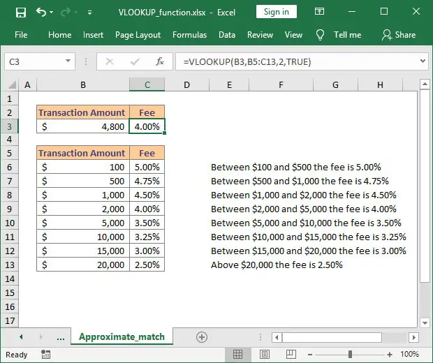
Whenever using an approximate match, your data must be sorted in ascending order by lookup value (in our case, the Transaction Amount). Otherwise, VLOOKUP will not retrieve the correct data.
Note: If you omit the match_type argument, Excel will use an approximate match by default but will retrieve the exact match if one exists.
As you become better at working in Excel, you will naturally feel the need to create more complex spreadsheets that better match your needs. This includes nesting functions.
One of the most used combos is nesting a VLOOKUP formula inside an IF statement so that the VLOOKUP formula is only triggered if certain conditions are met.
For example, there may be no point in looking for a sales bonus if the overall budgeted target is not met.
My recommendation is to play around with as many functions as possible. It’s the only way you will truly improve your Excel skills. And remember, if you need VLOOKUP help or have additional questions on how to use VLOOKUP, please let me know by posting a comment.

My name is Radu Meghes, and I'm the owner of excelexplained.com. Over the past 15+ years, I have been using Microsoft Excel in my day-to-day job. I’ve worked as an investment and business analyst, and Excel has always been my most powerful weapon. Its flexibility and complexity make it a highly demanded skill for finance employees. I launched excelexplained.com back in 2017, and it has become a trusted source for Excel tutorials for hundreds of thousands of people each year.
If you'd like to get in touch, you can contact me on LinkedIn.